-
Notifications
You must be signed in to change notification settings - Fork 3
Expand file tree
/
Copy path01_forming_questions_04_rstudio_cloud_tour.Rmd
More file actions
297 lines (143 loc) · 22.3 KB
/
Copy path01_forming_questions_04_rstudio_cloud_tour.Rmd
File metadata and controls
297 lines (143 loc) · 22.3 KB
1
2
3
4
5
6
7
8
9
10
11
12
13
14
15
16
17
18
19
20
21
22
23
24
25
26
27
28
29
30
31
32
33
34
35
36
37
38
39
40
41
42
43
44
45
46
47
48
49
50
51
52
53
54
55
56
57
58
59
60
61
62
63
64
65
66
67
68
69
70
71
72
73
74
75
76
77
78
79
80
81
82
83
84
85
86
87
88
89
90
91
92
93
94
95
96
97
98
99
100
101
102
103
104
105
106
107
108
109
110
111
112
113
114
115
116
117
118
119
120
121
122
123
124
125
126
127
128
129
130
131
132
133
134
135
136
137
138
139
140
141
142
143
144
145
146
147
148
149
150
151
152
153
154
155
156
157
158
159
160
161
162
163
164
165
166
167
168
169
170
171
172
173
174
175
176
177
178
179
180
181
182
183
184
185
186
187
188
189
190
191
192
193
194
195
196
197
198
199
200
201
202
203
204
205
206
207
208
209
210
211
212
213
214
215
216
217
218
219
220
221
222
223
224
225
226
227
228
229
230
231
232
233
234
235
236
237
238
239
240
241
242
243
244
245
246
247
248
249
250
251
252
253
254
255
256
257
258
259
260
261
262
263
264
265
266
267
268
269
270
271
272
273
274
275
276
277
278
279
280
281
282
283
284
285
286
287
288
289
290
291
292
293
294
295
296
297
```{r, include = FALSE}
ottrpal::set_knitr_image_path()
```
# RStudio and Projects
Remember [R](https://www.r-project.org/) is the main software that we are going to use to analyze data in this class. R is one of the two most popular languages for data science. We will learn a lot more about it throughout the courses, but here we are just going to use it to take a peak at the data you have created. R is a piece of software that is used for running computer code. [RStudio](https://www.rstudio.com/) is a company that makes a piece of software that works with R. RStudio makes it easier to create, save, share, and work with R code and data sets. RStudio is also useful for organizing projects and writing, organizing, and sharing your data science work.
If you have a more traditional laptop you can download and install R and RStudio on your laptop. However, the DataTrail Program will use RStudio through a web-based version of their software called Posit Cloud.
### Logging in to Posit Cloud
To use this software, open your web browser and navigate to the website <a href="https://posit.cloud/" target="_blank">Posit Cloud</a>.

You should see a screen that looks like this. You can click the button in the top right to log in.

When you click _Log In_ you will be offered options for Logging in, for our class you will log in with your Google Account so click on that option.

Then you will be asked to "Choose an account". Click on the Google account you have set up for this course.

You should now see a list of your projects. This is a list of the instructor's projects, your list will be different.

### Creating a new project
RStudio projects are where you will do your data science magic for this course and beyond!
To get started working on a new project, click on the "New Project" blue icon toward the top right. If you click the arrow next to `New Project`, you will notice there are multiple different options for creating a new project. For now choose `New Rstudio Project`, and we will discuss and use those other options later.

By starting a new project you'll be brought to a screen where three spaces are available.
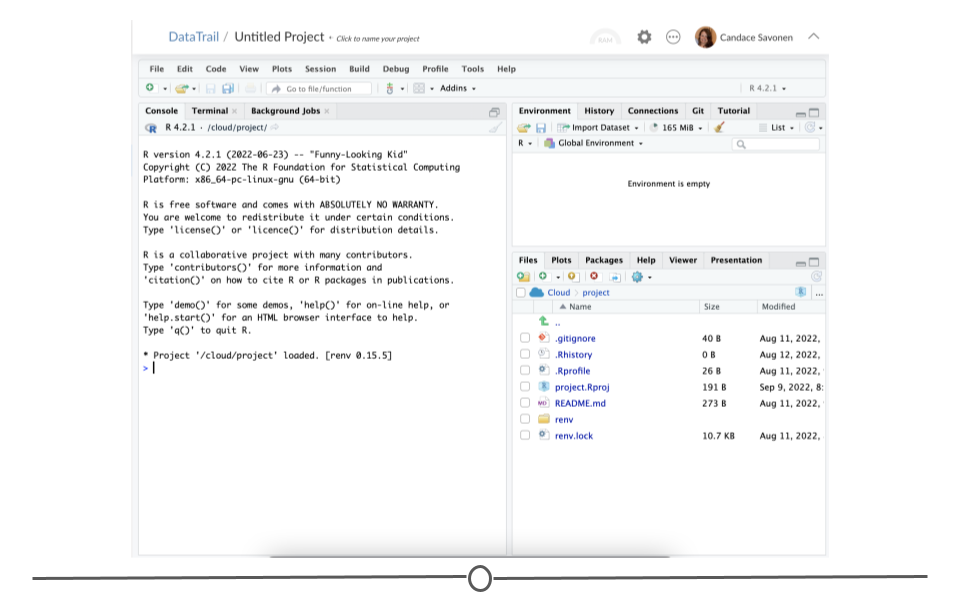
If you click on the name of the project - currently it will be _Untitled Project_ - then you can rename it.

To make things simple let's call it _my_first_project_. You will call it that by typing the name into the box for the project name.

If you want to see all the projects you have you can click on the words _Your Workspace_ at the top left of the screen.

If you want to return to a project, just click on the project name, for example by clicking on _my_first_project_.

Projects can be organized into Spaces. A space is just a place that lists out multiple projects.
You can click on the name of the DataTrail space in the upper left to see your projects there.

If you want to return to your original space, click again in the top left hand on the menu bar, then click on _Your Workspace_ to return to your main set of projects.
### The Tour
Now that we have a project. Return to your `my_first_project` so we can get oriented to the RStudio space.
We will go through each of the regions and describe some of their main functions, so follow along with each step and make sure you understand the function and how to access each part of Posit Cloud on your own. But, it would be impossible to cover everything that RStudio can do, so we urge you to explore Posit Cloud further on your own too!
To access the fourth space shown in the figure below, you'll have to start a new file. To do so, you'll click on File, hover over New File from the drop-down menu that appears, and then click "R Script" from the drop-down menu.
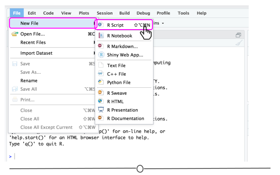
To open up a new file, you'll click on File, hover over New File from the drop-down menu that appears, and then click "R Script" from the drop-down menu.
This will open up a new R Script, which is currently called "Untitled," which you can see on the tab at the top left of the quadrant has just appeared.
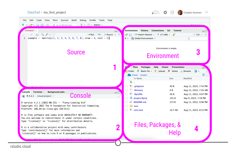
#### The menu bar
In addition to the four main quadrants, there is also a menu bar. The menu bar runs across the top of your screen and should have two rows. The first row should be a fairly standard menu, starting with "File" and "Edit." Below that, there is a row of icons that are shortcuts for functions that you'll frequently use.
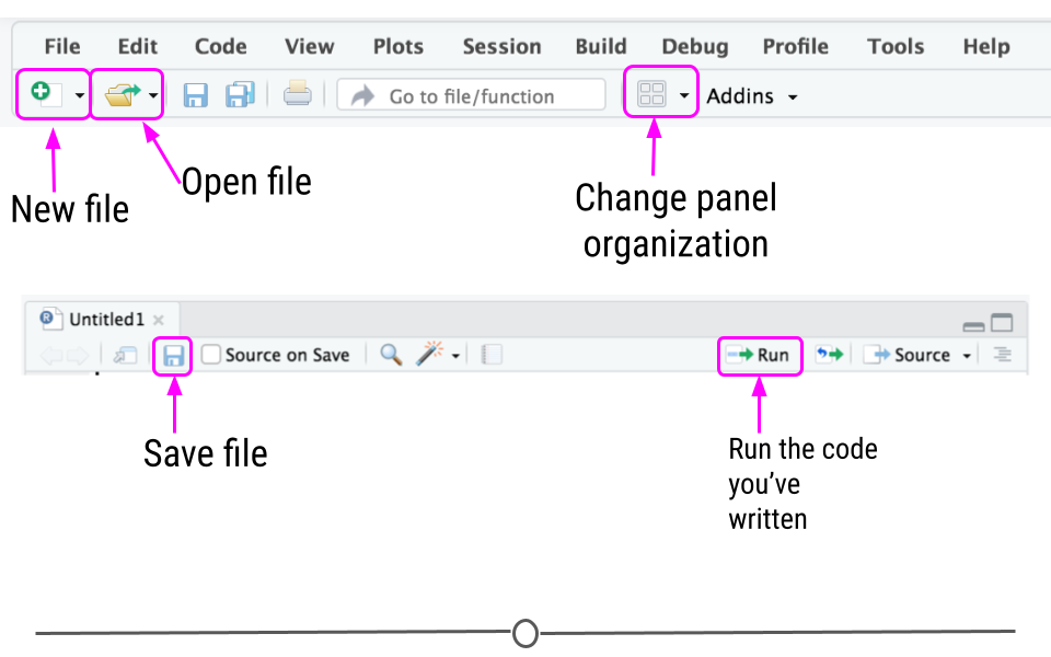
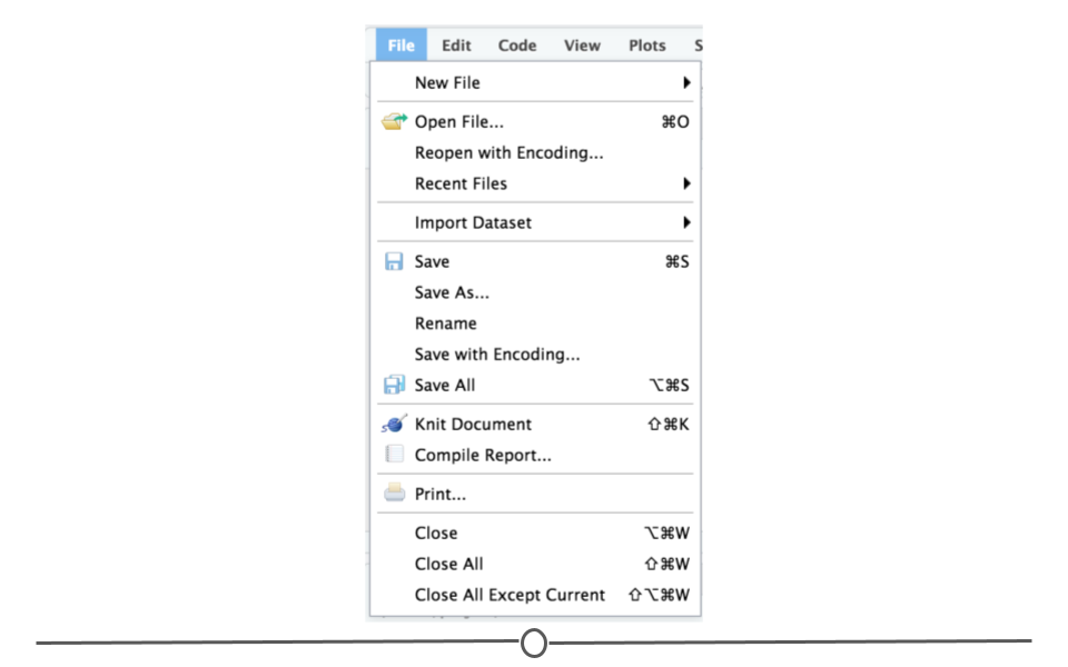
To start, let's explore the main sections of the menu bar that you will use. The first is the File menu. Here we can open new or saved files, save our current document, or close RStudio. As we saw earlier in this lesson, if you mouse over "New File", a new menu will appear that suggests the various file formats available to you. R Script and R Markdown files are the most common file types for use, but you can also generate R notebooks, web apps, websites, or slide presentations. If you click on any one of these, a new tab in the "Source" quadrant will open. We'll spend more time in a future lesson on R Markdown files and their use.
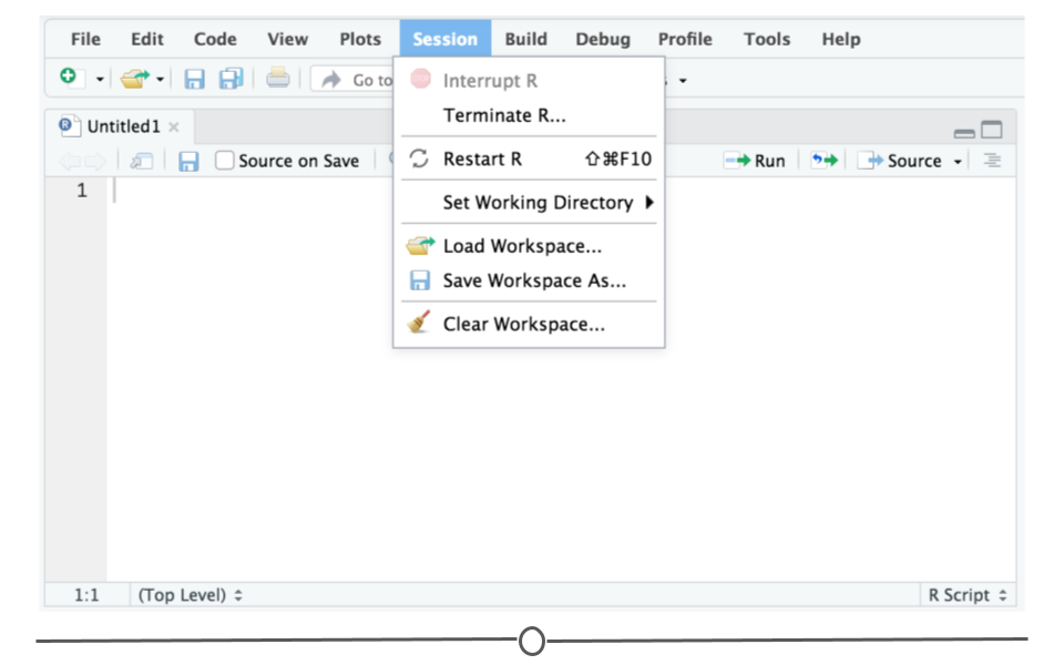
The Session menu has some R specific functions, in which you can restart, interrupt or terminate R - these can be helpful if R isn't behaving or is stuck and you want to stop what it is doing and start from scratch.
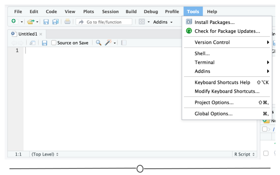
The Tools menu is a treasure trove of functions for you to explore. For now, you should know that this is where you can go to install new packages and set your options and preferences for how RStudio looks and functions. For now, we will leave this alone, but be sure to explore these menus on your own once you have a bit more experience with RStudio and see what you can change to best suit your preferences!
#### Console
When you first opened R, you were presented with the console. This is where you type and execute commands, and where the output of these commands is displayed.
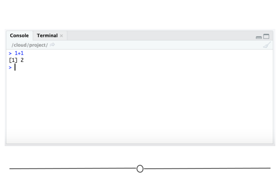
To execute your first command, at the `>` prompt, try typing `1 + 1`. Then, hit enter. You should see the output `[1] 2` below your command.
### Source: script editor panel
However, often you want to write code and save it so that you can open the code again and re-run it later. This saved file with code in it is referred to as a **script**. When you want to write code and save it in a script, you'll do this in the Source panel.
To get started in your script file, copy and paste the following into your Source quadrant (top-left).
```r
example <- matrix(c(1, 2, 3, 4, 5, 6, 7, 8), nrow = 4, ncol = 2)
```
To run this code, you *can't* just hit enter (as you were able to do in the Console). Hitting enter will just bring your cursor to the next line in the script. Instead, with your cursor in the line of code you want to run, you can click on "Run" at the top right of your script file. This will execute the code in the Console.
<div class = "notice">
Alternatively, to run code, with your cursor on the line of code you'd like to run, you could **hit 'ctrl + enter' to run that line of code**. This will save you *a lot* of time as you start writing a lot of code and analyzing data. Practice this keyboard shortcut now!
</div>
What this code does is create an object (we'll define what that is soon!) called 'example' that has the numbers 1 through 8 in four different rows and two different columns. To see what this object looks like, we'll take a look at the environment quadrant of Posit Cloud.
#### Environment (& History)
To view this object we've just created, you'll first want to ensure that the object was created. In the Environment quadrant, you should see that 'example' is now there. The object was created!
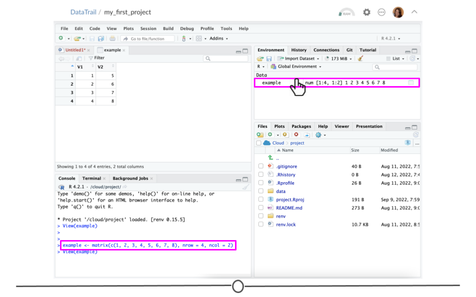
Then, just click anywhere on the "example" line, and a new tab on the Source quadrant should appear, showing the matrix you created.
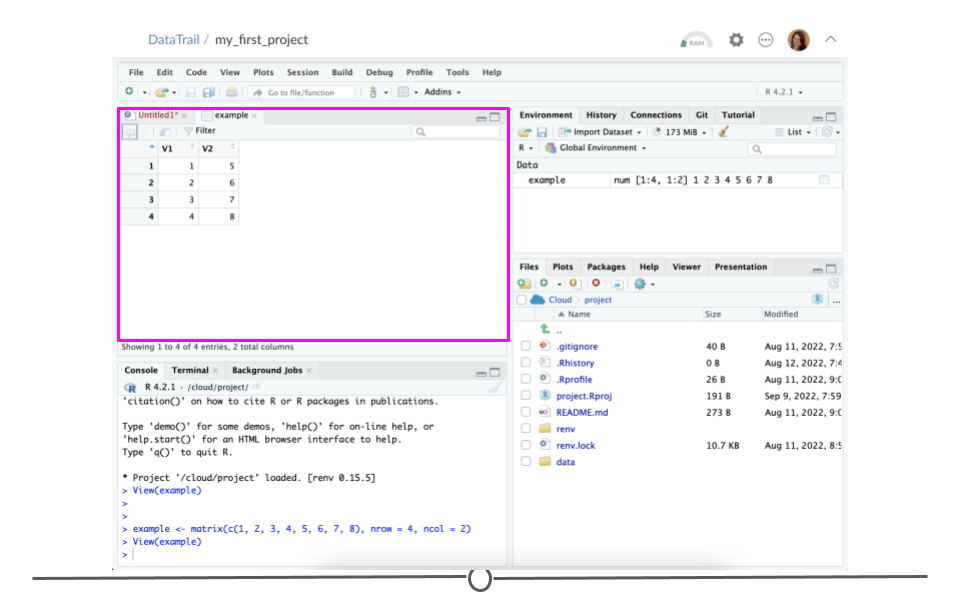
Posit Cloud also tells you some information about the object in the environment, like whether it is a list or a data frame or if it contains numbers, integers or characters. This is very helpful information to have as some functions only work with certain classes of data. We'll get into the details of all this later, but for now, knowing that this information is in the Environment tab is enough.
The quadrant has two other tabs running across the top of it. We'll just look at the History tab now. Your history tab should look something like this:
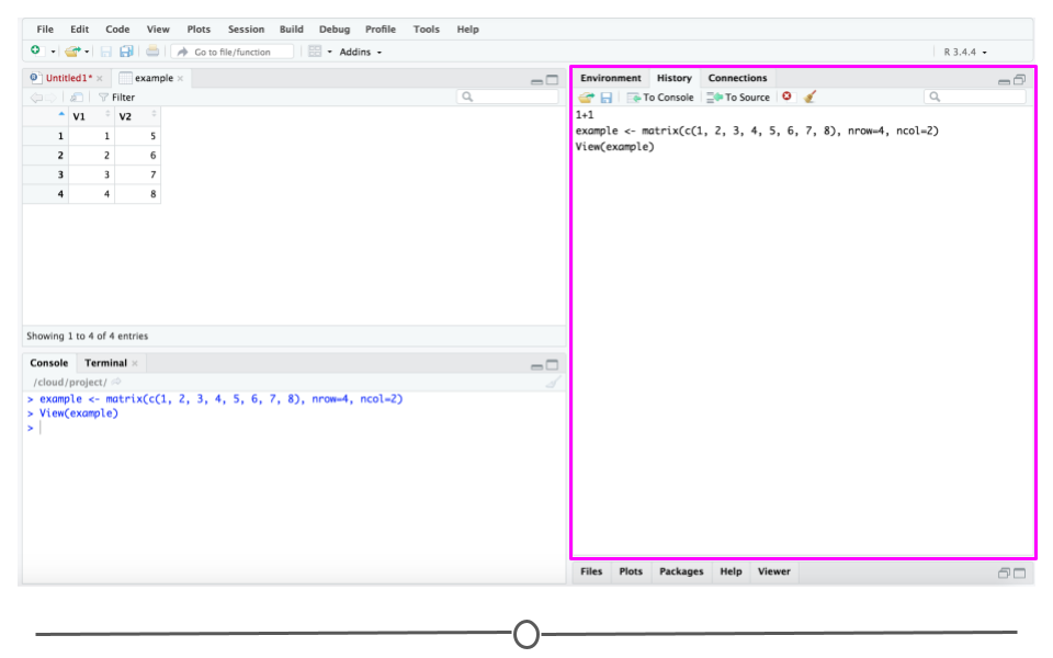
Here you will see the commands that we have run in this session of R. If you click on any one of them, you can click "To Console" or "To Source" and this will either rerun the command in the console, or will move the command to the source, respectively.
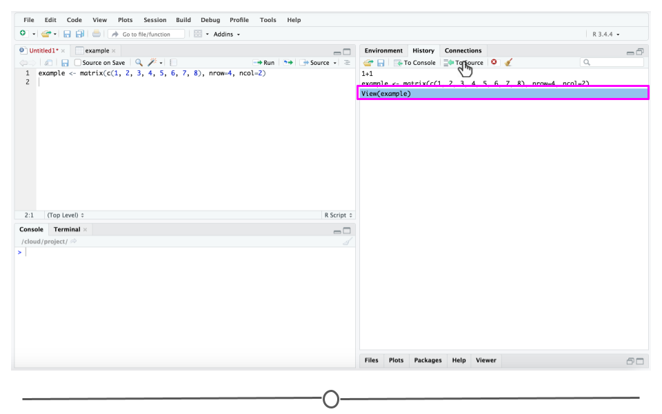
Do so now for your `View(example)` command and send it to source by clicking "To Source".
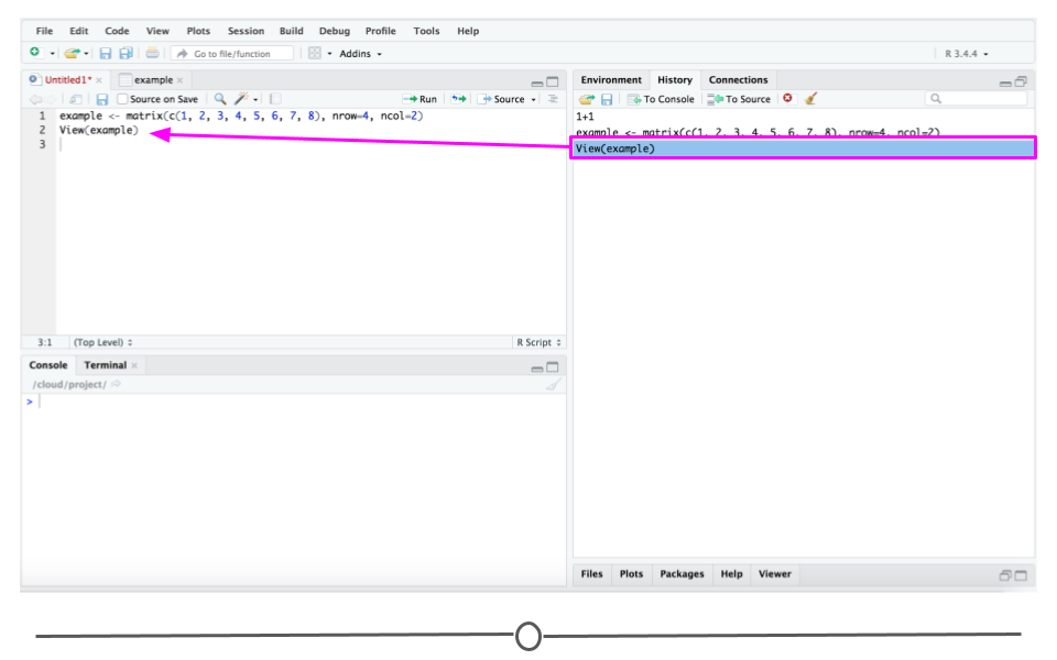
This line of code is now in your Source document. When you save this document, you'll also have this line of code saved for future use.
#### Saving Files
Now that you've created a script with code in it, you likely want to save it. To do so, you'll want to click on the save icon.
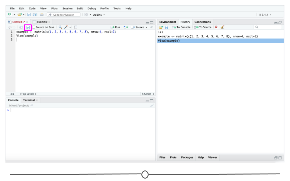
In Posit Cloud this will open a Save File window.
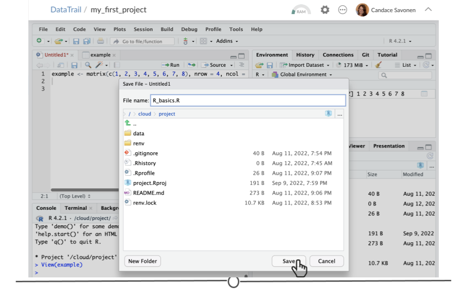
Type in the name you want for this file. For now, let's call it 'R_basics.R'. It's important that it ends in a `.R` since that is the file type we are working with, but we'll return to this concept later.
Click the `Save` button.
The file name 'R_basics.R' will now show up in the tab at the top of the R Source quadrant.
#### Making a new folder
Now let's create a new folder for storing our data that we'll need. In the bottom right quadrant of your console, click the `New Folder` icon.
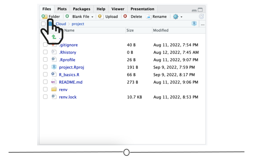
We'll name this folder "data" by typing it in the box and clicking "OK".
To move in and out of folders, you can click on folder names in the `Files` pane.
### Files/Help/Plots/Packages/Viewer
#### Files
You can also see where this file is saved using the fourth and final quadrant in Posit Cloud that we'll discuss. In this final quadrant you'll see five tabs: Files, Plots, Packages, Help, and Viewer.
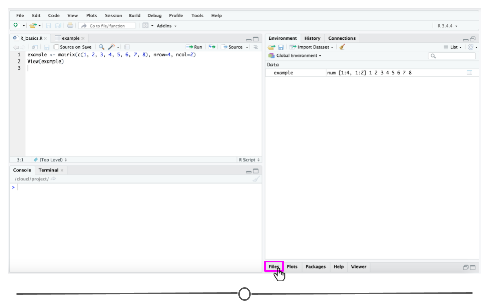
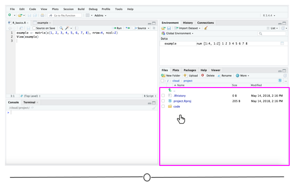
In Files, you can see everything in your Posit Cloud project by moving around. You should now be able to see the data folder you just created.
Clicking on that folder, and create another folder within it called `raw_data`
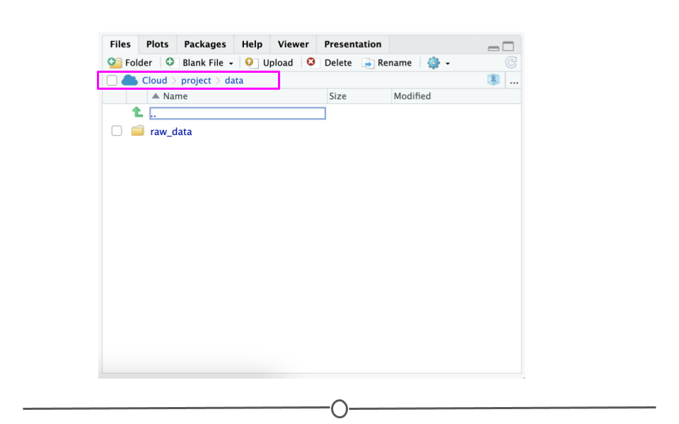
Note that you can see on the top of this bar what folder this folder is in. This is called a file path and we'll get into this more later.
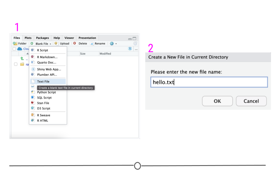
Let's create some fake data to store in this `raw_data` folder. Click the `New Blank File` button and create a Text file that is called `hello.txt` and save it to this `raw_data` folder.
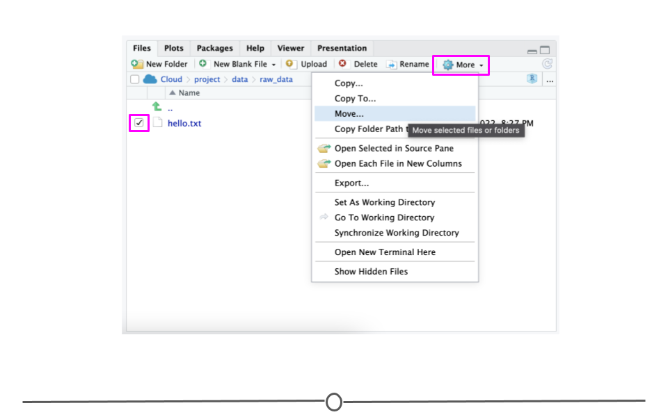
After you save a file in a folder, if you realize it's not where you wanted it, you do have the option to move it around. To do so, click on the check box of the file you want to move, and click on the "More" icon to expose options. Click through these to move your file to where you actually wanted it.
#### Plots
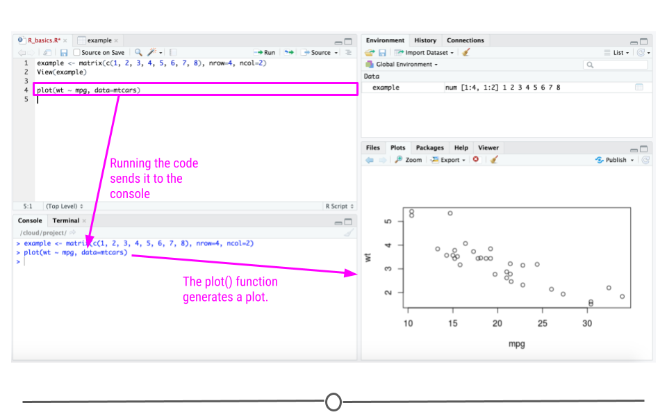
In the Plots tab, if you generate a plot with your code, it will appear here. You can use the arrows to navigate to previously generated plots. The Zoom function will open the plot in a new window, that is much larger than the quadrant. Export is one way to save the plot. (Saving plots will be discussed in more detail in a future lesson.) The broom icon clears all plots from memory.
#### Packages
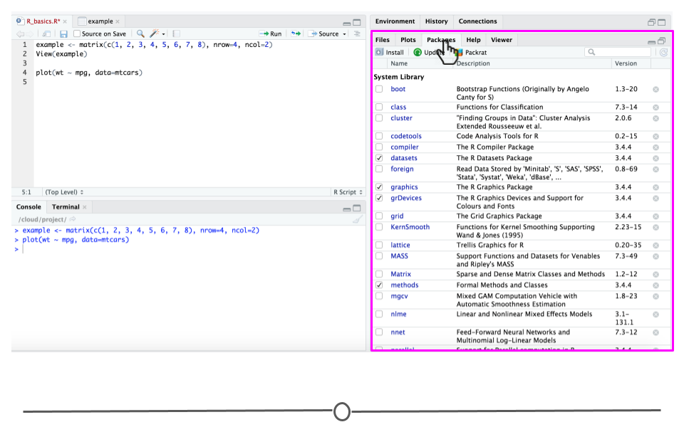
The Packages tab will be explored more in depth in the next lesson on R packages. Here you can see all the packages you have installed, load and unload these packages, and update them.
#### Help
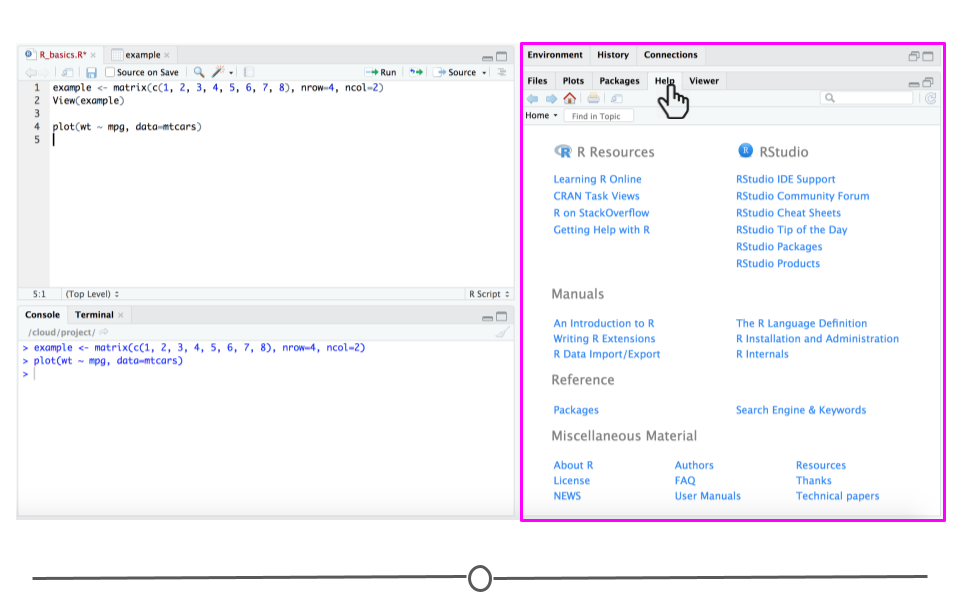
The Help tab is where you find the documentation for your R packages and various functions. In the upper right of this panel there is a search function for when you have a specific function or package in question. Navigating this tab will be discussed in more detail in a later lesson in this course.
### Swirl
Throughout the DataTrail curriculum, we'll be using something called [Swirl modules](https://swirlstats.com/) to practice the R code learned in many of the lessons. These modules can be run in R.
To make sure that you're comfortable using Swirl, we'll go through the steps on where to go to run Swirl and how to work through a module. This will be important as many of the quizzes accompanying these lessons will require you to use Swirl. Follow the steps in this section of the lesson to get started with your first Swirl module!
Following the [steps we just did to open a new project](https://datatrail-jhu.github.io/DataTrail/rstudio-and-projects.html#creating-a-new-project), open up a new project in R and call it `swirl_practice_yourname` but replace `yourname` with your own name.
In this new project, run the following code to install swirl:
```r
install.packages("swirl")
```
Any time you are within this space and supposed to complete a swirl module you'll start by first loading the swirl package (it has already been installed in that space for you) and running the command `swirl()`:
Run the following code to start up swirl. Note that lines that start with `#` aren't actually run by R.
```r
## load package
library(swirl)
## start swirl
swirl()
```
As a reminder, to run code, with your cursor on the line of code you'd like to run, you can **hit 'ctrl + enter' to run that line of code**. Similarly, if there are multiple lines you want to run, you can highlight the lines you want to run and again hit 'ctrl + enter' to run those lines of code.
This will bring up a prompt asking you what swirl should call you. Type your first name as a response here and hit "enter."
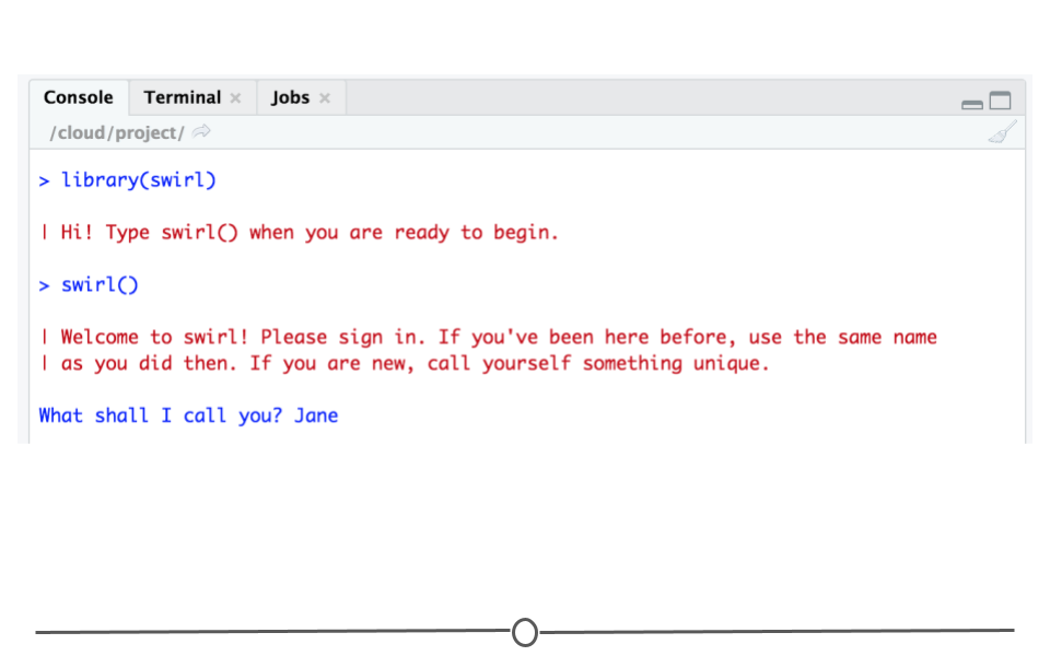
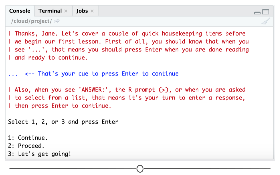
Swirl will often send you some text to read. *Always read the text* as this text will help explain the background information you need *or* will provide you with information you need to answer the question. At this point, swirl is explaining that when you see `...`, that's when you should press "enter" to continue.
When you see `>` or a list of options (like `1:`, `2:`, `3`), that lets you know swirl is looking for something from you! When you see `>` that's a prompt letting you know swirl is expecting you to write some code. When you see a list of options, those are the possible answers to a question you're being asked. In these cases, you'll want to select the number corresponding to the right answer. For this practice in swirl, select 1, 2, or 3 and press enter.
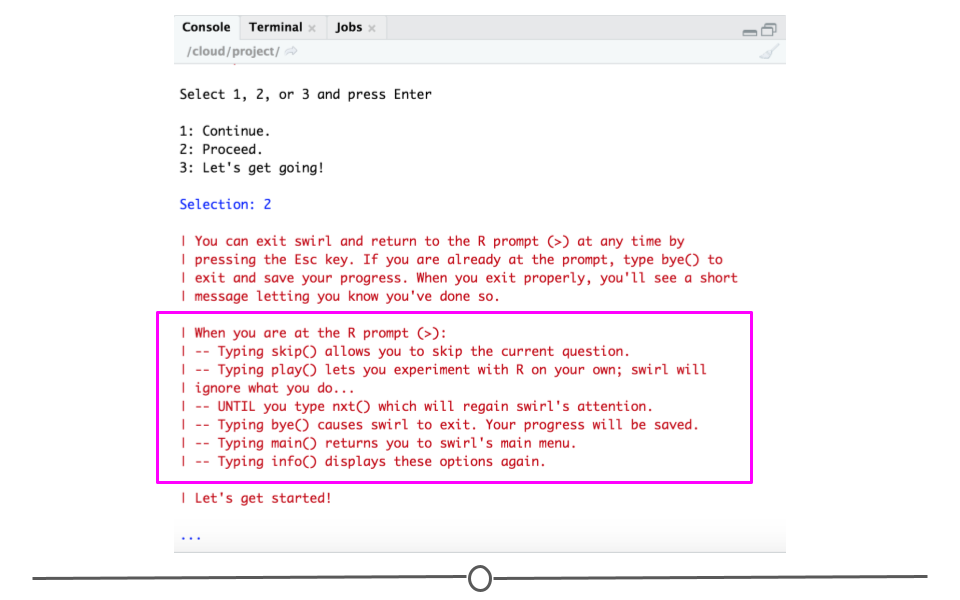
You'll then be given a number of options that you can use within `swirl` whenever you see the `>` prompt. Read the list here, but know that `info()` gives you this list of options again, `main()` returns you to swirl's main menu, and `bye()` saves your progress but exits swirl.
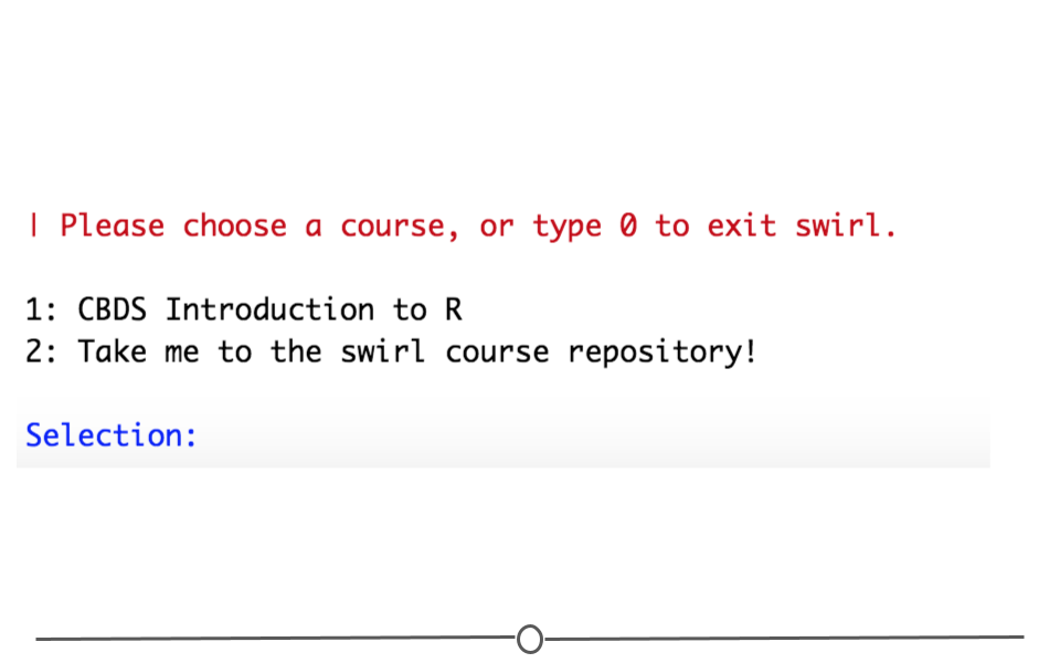
After this, you will be shown a list of courses. The list will be longer than what you see here, but we're showing this simple example to demonstrate that if you wanted to start on the course "DataTrail Introduction to R", you would type 1. You'll be told which course to select throughout the course set.
Note that for each quiz question you complete in `swirl`, upon completion, you'll receive a code. This code is to be entered as the answer to the quiz question on Leanpub.
That's a basic introduction to using `swirl`. You'll have lots of quiz questions that require you to use swirl in this course, so be sure to walk through this introduction on Posit Cloud now and get comfortable navigating within swirl.