Anistroph

Multi-Domain Predictive Analytics with AI Agent Access

Anistroph connects dataset-specific predictive models to shared services for prediction, explainability, evaluation, multidimensional analysis, and AI-agent access.

Anistroph Through Claude

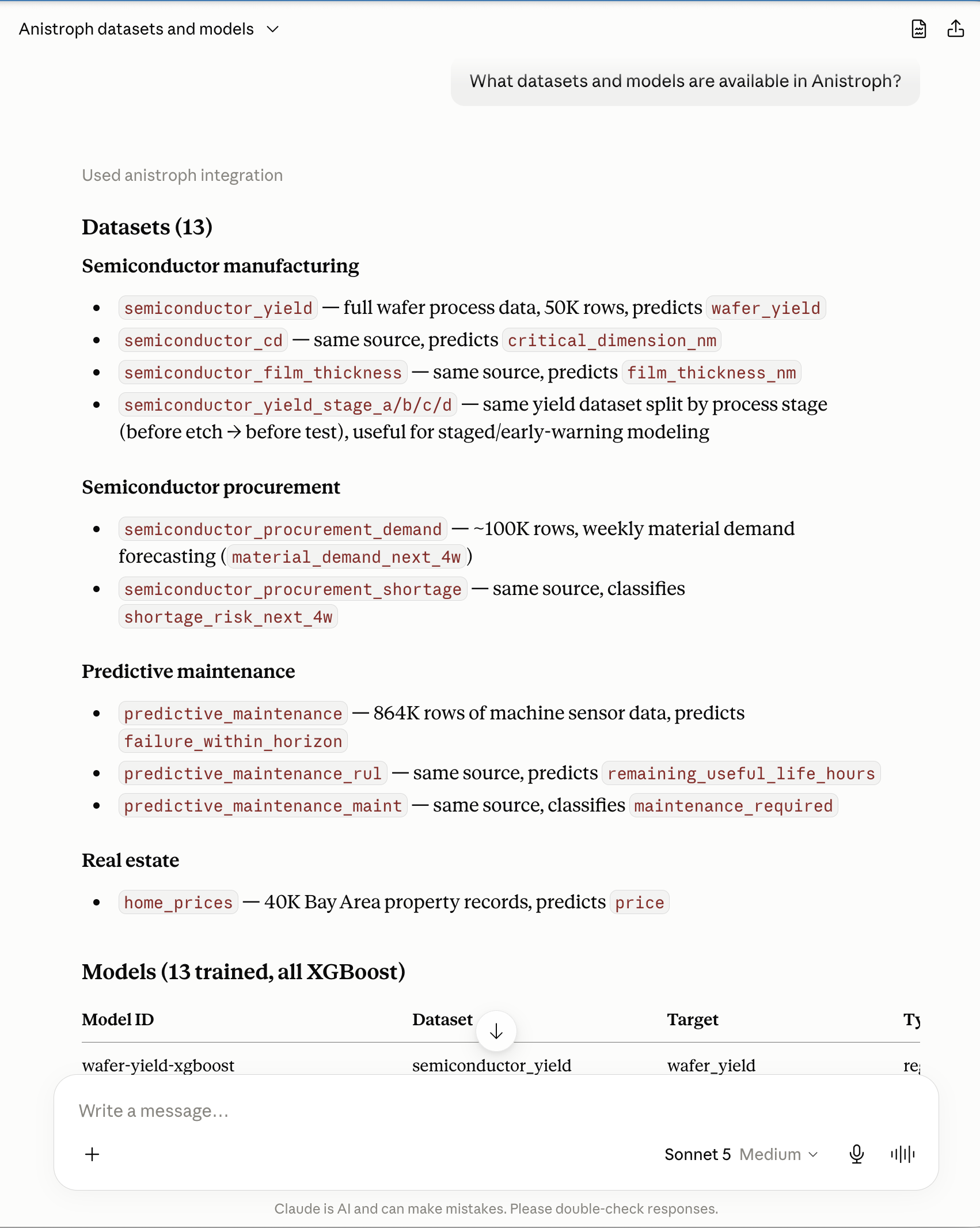
"What datasets and models are available in Anistroph?"

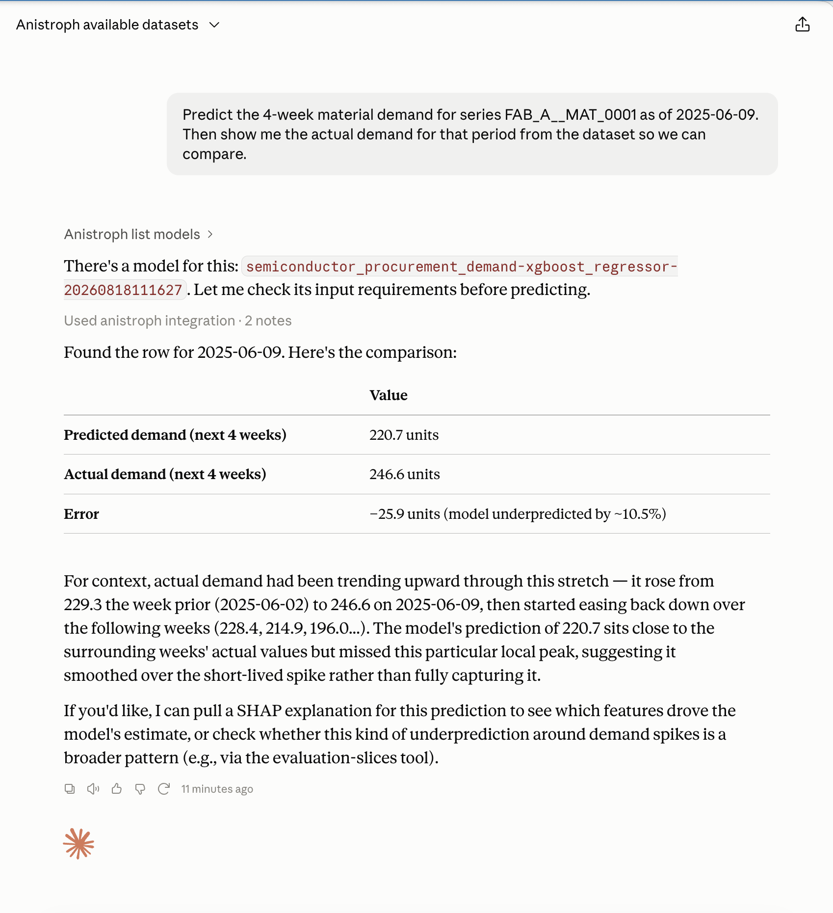
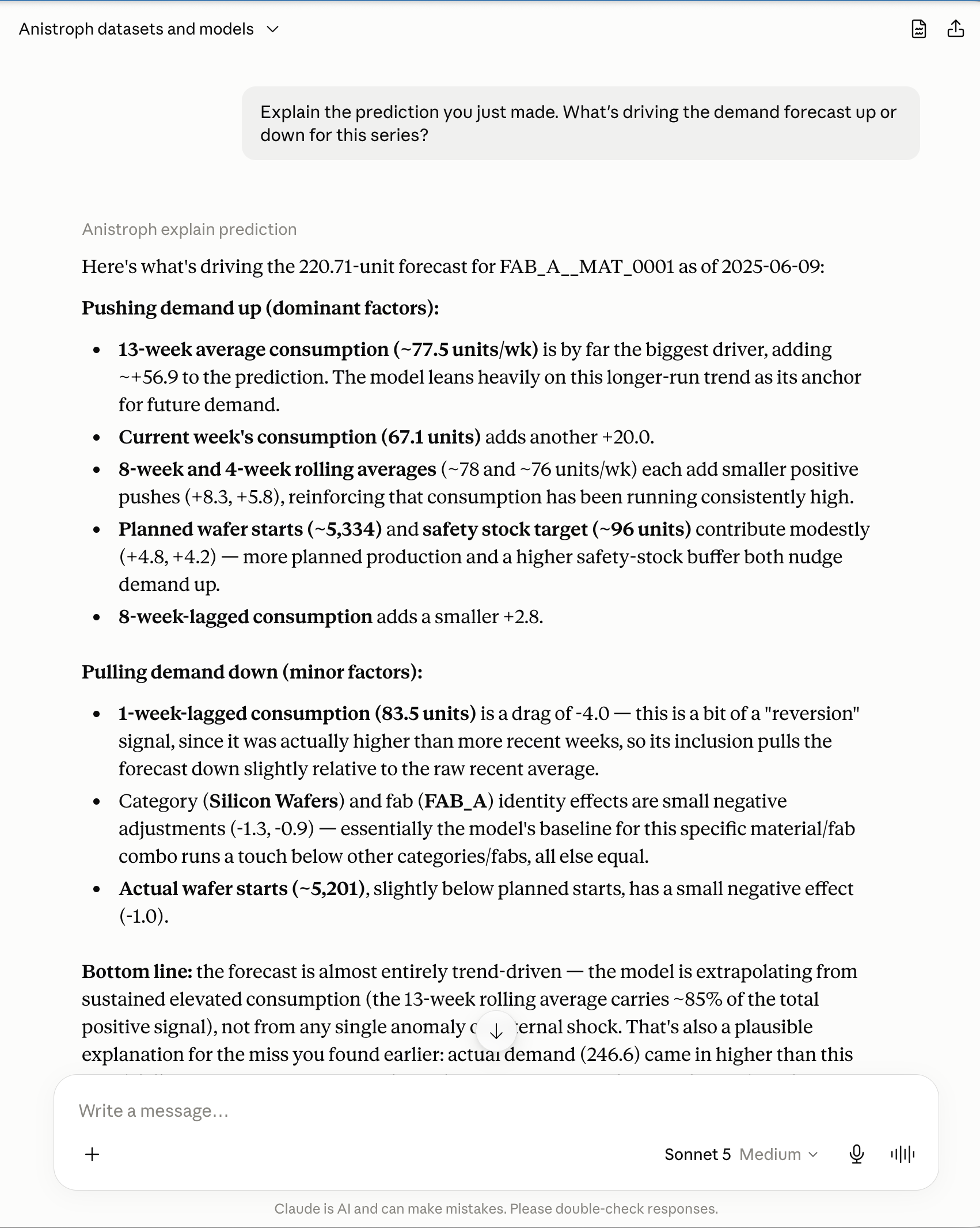
"Predict the 4-week material demand for FAB_A__MAT_0001 as of 2026-07-06. Then show me the actual demand so we can compare."

"Explain what's driving the demand forecast up or down."

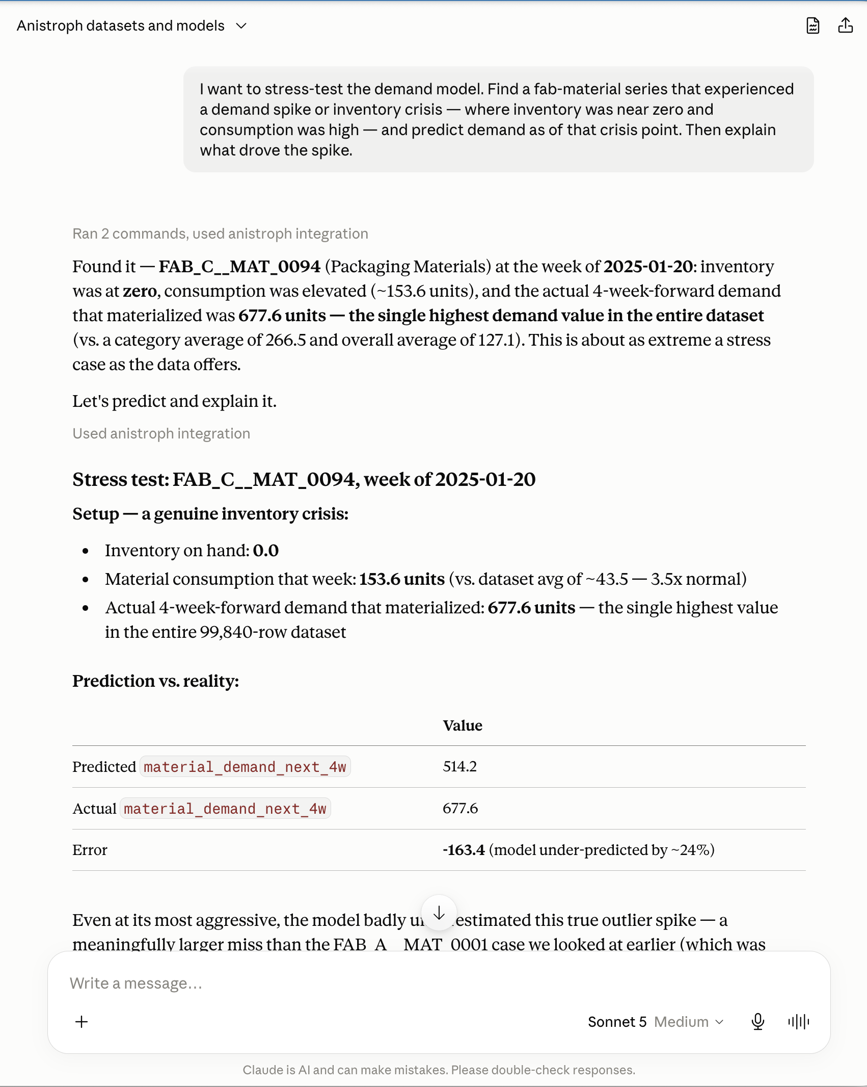
"Find a fab-material series that experienced a demand spike or inventory crisis , predict demand at that point, and explain what drove the spike."

Claude and other AI agents can discover → understand → execute through MCP. Anistroph performs the underlying prediction, explanation, evaluation, and analysis through its shared runtime.

MCP access: Anistroph includes an MCP server that can run locally or be deployed with the application. MCP-compatible clients can connect to their own Anistroph environment through stdio or Streamable HTTP.

Shared Runtime, Different Prediction Problems

Different datasets retain their own schemas, features, targets, preprocessing, and models while using the same training, prediction, explanation, evaluation, and analytical services.

The same runtime supports semiconductor manufacturing, predictive maintenance, materials procurement, and additional domains without rebuilding those shared services.

MCP, REST/OpenAPI, and the Web UI use the same runtime, allowing agent-driven predictions and analyses to be independently reproduced when validation is required.

Predictive Analytics — Claude MCP in Action

Discovering datasets and models	Predicting material demand
Explaining the prediction with SHAP	Stress-testing a real inventory crisis

Core Features

• Multi-Domain Predictive Runtime --- Different datasets retain their own schemas, features, targets, preprocessing, and models while sharing prediction, explanation, evaluation, and analysis services.
• AI Agent Access through MCP --- Claude and other MCP-compatible agents can discover datasets and models, inspect model contracts, and invoke prediction, explanation, evaluation, and analysis through stdio or Streamable HTTP.
• Self-Describing Models --- Model contracts expose required inputs, prediction mode, and temporal requirements such as as_of and inference history.
• Temporal & Records-Based Prediction --- Supports direct source-record inference and temporal entity lookup with rolling feature reconstruction from historical data.
• Multiple Targets & Process Stages --- A source dataset can support different prediction targets and task types, or models for the same target at different process stages.
• SHAP Explainability & One-Hot Feature Normalization --- Maps SHAP contributions from one-hot encoded features back to their original source features and values.
• Multidimensional Analysis & Evaluation --- Analyzes observed outcomes and model performance across 1-, 2-, and 3-dimensional populations.
• Cross-Interface Validation --- MCP, REST/OpenAPI, and the Web UI use the same shared runtime, allowing agent-driven operations to be independently reproduced and validated.
• Parametric Search --- Datasets can declare a structured search contract with searchable fields, units, aliases, and semantic filters (e.g. "supports 55°C" → range-containment). Agents discover the contract, normalize natural-language requirements, and apply deterministic filters via the same shared service layer.
• External A2A Integration --- Anistroph can hand off context to externally-hosted AI agents (e.g. Aina-Veris for datasheet RAG) via A2A JSON-RPC. External tools are defined in a tool registry and exposed through both MCP and REST. Aina-Veris is used as the reference implementation but is not a hard dependency — any A2A-compatible system can be configured.

Anistroph is a reference architecture. The included synthetic datasets and models demonstrate how the components fit together rather than claiming validation across every potential domain.

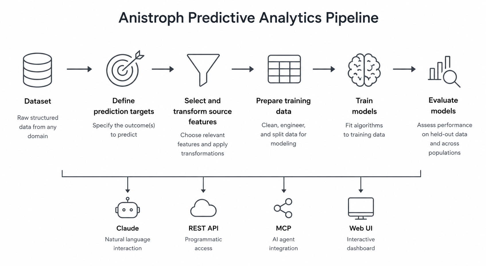
The Anistroph predictive analytics pipeline — from dataset configuration through shared services to MCP, REST, and Web UI interfaces.

---

Reference Datasets

Anistroph includes synthetic reference datasets across multiple domains to exercise different architectural capabilities. The primary reference implementations cover semiconductor manufacturing, predictive maintenance, semiconductor materials procurement, and semiconductor memory parametric search, with a lightweight real-estate dataset providing an additional cross-domain regression test.

Reference domain	What it exercises
Semiconductor Manufacturing	Multiple regression targets, process-stage prediction, explainability, multidimensional analysis and evaluation
Predictive Maintenance	Temporal sensor data, classification + regression, rolling features, equipment-health prediction
Semiconductor Materials Procurement	Temporal prediction, rolling demand features, 4-week demand forecasting, shortage-risk classification
Semiconductor Memory	Parametric product search with semantic filters (range-containment, industrial temperature), search contract discovery, predict-on-search ranking by supply risk / lead time
Real estate	Lightweight non-manufacturing regression example for cross-domain validation

The same source data can support multiple target configurations. For example, the semiconductor manufacturing source supports separate yield, critical-dimension, and film-thickness models, each with its own feature/target configuration, partitions, metrics, and persisted model artifacts.

Shipped Dataset Configurations

Anistroph ships 16 reference dataset configurations. After setup, all 16 should appear under Web UI → Datasets → Registered Datasets.

Domain	Dataset ID	Purpose
Predictive maintenance	predictive_maintenance	Failure-within-horizon classification
Predictive maintenance	predictive_maintenance_rul	Remaining-useful-life regression
Predictive maintenance	predictive_maintenance_maint	Maintenance-required classification
Semiconductor manufacturing	semiconductor_yield	Wafer-yield regression
Semiconductor manufacturing	semiconductor_cd	Critical-dimension regression
Semiconductor manufacturing	semiconductor_film_thickness	Film-thickness regression
Semiconductor manufacturing	semiconductor_yield_stage_a	Stage A wafer-yield prediction
Semiconductor manufacturing	semiconductor_yield_stage_b	Stage B wafer-yield prediction
Semiconductor manufacturing	semiconductor_yield_stage_c	Stage C wafer-yield prediction
Semiconductor manufacturing	semiconductor_yield_stage_d	Stage D wafer-yield prediction
Real estate	home_prices	Home-price regression
Semiconductor procurement	semiconductor_procurement_demand	Four-week demand regression
Semiconductor procurement	semiconductor_procurement_shortage	Four-week shortage-risk classification
Semiconductor memory	semiconductor_memory	Parametric catalog search and analysis
Semiconductor memory supply	semiconductor_memory_supply_risk	Four-week supply-risk classification
Semiconductor memory supply	semiconductor_memory_supply_lead_time	Four-week lead-time regression

The YAML configurations are version-controlled under datasets/. Generated source data, partitions, and artifacts/dataset_registry.json are local runtime artifacts created by setup; the registry is intentionally excluded from Git because it can contain machine-specific paths.

Trained Reference Models

Held-out evaluation metrics for the shipped reference models:

Domain	Target	Task	Held-out metric
Semiconductor Yield	wafer_yield	Regression	R² = 0.81
Semiconductor CD	critical_dimension_nm	Regression	R² = 0.89
Semiconductor Film Thickness	film_thickness_nm	Regression	R² = 0.98
Predictive Maintenance — Failure	failure_within_horizon	Classification	ROC-AUC = 0.85, F1 = 0.61
Predictive Maintenance — Maintenance	maintenance_required	Classification	ROC-AUC = 1.00, F1 = 0.94
Predictive Maintenance — RUL	remaining_useful_life_hours	Regression	MAE = 27.9h
Home Prices	price	Regression	R² = 0.97
Procurement — Demand	material_demand_next_4w	Regression	R² = 0.96, MAE = 14.0
Procurement — Shortage Risk	shortage_risk_next_4w	Classification	ROC-AUC = 0.99, F1 = 0.90
Memory Supply Risk	supply_risk_next_4w	Classification	ROC-AUC = 0.999, F1 = 0.979
Memory Supply Lead Time	lead_time_next_4w_days	Regression	R² = 0.996, MAE = 1.1d

Models are trained on the train partition and evaluated on the held-out evaluation partition (most recent 20% for temporal datasets, random 20% for non-temporal). The two never overlap.

Note: These metrics are from synthetic reference datasets designed to exercise Anistroph's architecture and workflows; they are not benchmarks of expected real-world model performance.

For dataset-specific prompts and worked examples, see the Setup & Usage Guide.

---

Install / Setup

The quickest path is to install Anistroph, generate/register the reference datasets, and connect Claude Desktop through MCP stdio.

1. Clone

git clone https://github.com/vrraj/anistroph
cd anistroph

2. One-shot setup

make install

make install:

• checks for libomp on macOS, required by XGBoost;
• creates .venv and installs Anistroph in editable mode;
• creates .env from .env.example;
• generates and registers the sixteen reference dataset configurations;
• prints a ready-to-paste Claude Desktop MCP configuration with absolute paths.

3. Connect Claude Desktop

Paste the generated configuration into:

~/Library/Application Support/Claude/claude_desktop_config.json

It will look like:

{
  "mcpServers": {
    "anistroph": {
      "command": "/absolute/path/to/anistroph/.venv/bin/python",
      "args": ["-m", "backend.integrations.mcp.server"],
      "cwd": "/absolute/path/to/anistroph"
    }
  }
}

Restart Claude Desktop and try:

"List all Anistroph datasets and models."

"Predict wafer yield for WAFER_015000 and explain what pushed it up or down."

"Where does the wafer-yield model perform worst across product, tool, and chamber combinations?"

MCP stdio does not require the FastAPI server to be running.

4. Optional: start the service

Start the service when you want REST/OpenAPI, MCP Streamable HTTP, or the Web UI:

make start-native    # local .venv
# or
make start           # Docker Compose

Access points:

• MCP stdio: Claude Desktop / Claude CLI --- no server required
• MCP Streamable HTTP: http://localhost:9500/mcp
• REST / OpenAPI: http://localhost:9500/docs
• Web UI: http://localhost:9500

For the full installation, MCP setup, examples, and troubleshooting guide, see Setup & Usage.

Troubleshooting: Datasets Are Missing from the UI

The Datasets UI lists entries from the local artifacts/dataset_registry.json. If the list is empty or shows fewer than 16 datasets, rebuild the local registry.

For a fresh clone, or when source data may also be missing, run:

make setup

If the source CSV/Parquet files already exist and only the registry is missing or incomplete, use the faster registration-only path:

.venv/bin/python scripts/setup_datasets.py --skip-gen

The command should finish with:

Total registered: 16 dataset(s).

Then open the Datasets tab and click Refresh. The standard Docker and native start commands also run this idempotent setup automatically, so subsequent starts check the registry and skip datasets that are already registered.

---

Core Architecture Concepts

Dataset and Model Isolation

Each dataset declares its own schema and predictive contract through configuration rather than embedding domain concepts into the shared runtime.

             Dataset
                │
                ▼
          DatasetSpec
                │
       ┌────────┼────────┐
       ▼        ▼        ▼
 FeatureSpec TargetSpec ModelSpec
       │        │        │
       └────────┼────────┘
                ▼
         Common Pipeline

• DatasetSpec --- columns, types, roles, entity keys, and optional time keys.
• FeatureSpec --- model inputs and transforms, including categorical encoding and temporal rolling features.
• TargetSpec --- target semantics such as regression, classification, or future event.
• Model artifacts --- trained model, feature metadata, preprocessing contract, feature order, and evaluation metrics.

Dataset-specific preparation can be added where a domain requires it without placing domain logic inside shared training, inference, analysis, or transport services.

Shared Predictive Runtime

Once trained, models participate in the same runtime regardless of domain:

• Predict --- run inference for an entity or source-feature record.
• Explain --- identify the source features that contributed most to an individual prediction.
• Evaluate --- measure persisted-model performance against held-out data, overall or for selected populations.
• Analyze --- slice and compare observed data and discover unusual multidimensional populations.

This separation is what allows semiconductor, equipment-health, procurement, home-price, and future datasets to use the same service contracts.

---

Modeling and Evaluation

Models Currently Implemented

---

Task Models Typical output

---

Classification XGBoost Classifier, probability / class Logistic Regression

Regression XGBoost Regressor, continuous value Linear Regression
(Ridge)

TargetSpec declares the prediction task. When a model type is not explicitly supplied, the task determines the default model family and evaluation metrics.

Held-Out Evaluation

Datasets are partitioned at registration into training and evaluation partitions. Temporal datasets split chronologically; non-temporal datasets shuffle with a fixed seed.

Training uses only train.parquet. Evaluation runs the persisted model against evaluation.parquet without fitting or modifying the model.

Regression: MAE, MSE, RMSE, R², MAPE, max error, median absolute error, p95 absolute error, mean prediction error, and baseline comparison.

Classification: ROC-AUC, PR-AUC, precision, recall, F1, and confusion matrix.

Multidimensional Model Evaluation

Aggregate metrics can hide populations where a model performs materially differently. Anistroph can evaluate model error across 1-, 2-, and 3-dimensional categorical combinations.

Overall Evaluation
       │
       ├── Aggregate metrics
       │
       └── Multidimensional Evaluation
                    │
          ┌─────────┼──────────────┐
          ▼         ▼              ▼
       Product   Product × Tool   Product × Tool × Chamber

This separates two questions:

• Multidimensional analysis: where is an observed outcome unusually high or low?
• Multidimensional model evaluation: where does the model perform unusually well or poorly?

---

Temporal Prediction and Rolling Forecasts

Temporal models can use history-dependent features without retraining for every new prediction period.

For example, a procurement model may predict material demand over the next four weeks using current inventory, supplier metrics, production plans, and recent consumption trends.

Recent Entity History
        ↓
Current Rolling Features
        ↓
Persisted Model
        ↓
Future Prediction

Anistroph separates:

• Training --- learns relationships between features and outcomes.
• Temporal feature calculation --- reconstructs current rolling/history-based inputs from entity history.
• Forecast horizon --- defines the future period represented by the target.

For a rolling four-week target:

As of Week 10 → predict Weeks 11–14
As of Week 11 → predict Weeks 12–15
As of Week 12 → predict Weeks 13–16

The as_of point is the boundary of known information. History-dependent transforms use only observations available through that point, preventing future leakage.

The required inference history is derived from the model's configured feature windows. New observations can therefore produce new predictions with updated feature values while the persisted model remains unchanged.

Temporal vs Non-Temporal Datasets

Anistroph distinguishes two dataset types based on whether a time_key is declared in the YAML:

	Temporal dataset	Non-temporal dataset
YAML	time_key: <column>	time_key omitted or null
Examples	Procurement (weekly), Predictive Maintenance (5-min sensor)	Semiconductor Yield (per wafer), Home Prices (per listing)
Splitting	Chronological (oldest → train, newest → eval)	Random with fixed seed
Rolling transforms	Available (mean, std, slope, delta over time windows)	Not applicable
Prediction	Entity lookup loads history up to as_of date to build rolling features	Entity lookup fetches single row; records mode also available

A dataset can have a timestamp column for chronological splitting without being "temporal" in the forecasting sense. The key distinction is whether the model's feature transforms include rolling windows — if they do, the runtime requires entity_id + timestamp for prediction so it can load historical observations. The anistroph_get_model_inputs tool exposes this via requires_timestamp and prediction_mode, so agents know which inputs to request.

For the full treatment of as_of, rolling feature reconstruction, inference history, forecast horizons, and retraining, see Setup & Usage → Temporal Prediction.

---

Explainability

Anistroph exposes a common explanation interface while allowing the explanation method to depend on the model family.

XGBoost / TreeSHAP

XGBoost classification and regression models use SHAP TreeExplainer (TreeSHAP). Contributions are signed, showing which inputs pushed an individual prediction higher or lower.

Source-Feature Normalization

Preprocessing can expand one source field into several model features:

product_id = PROD_B

        ↓ one-hot encoding

product_id__PROD_A = 0
product_id__PROD_B = 1
product_id__PROD_C = 0

        ↓ SHAP + normalization

feature = product_id
value   = PROD_B
impact  = summed contribution

anistroph_explain_prediction groups one-hot SHAP values back to the original source feature and returns the original input value. Raw per-category contributions remain available in a detail field for debugging.

Models without TreeSHAP support currently use an importance-weighted fallback and identify the method through explanation_method.

An explanation describes why the model produced a prediction; it is not treated as proof that a feature physically caused the observed outcome.

---

Multidimensional Discovery

Prediction and explanation are complemented by deterministic analysis of the underlying dataset.

Anistroph can slice data by one, two, or three dimensions and aggregate metrics using mean, sum, min, max, count, standard deviation, or median. find_interesting_slices searches categorical combinations and ranks populations by deviation from the overall baseline while enforcing a minimum sample size.

                 DATA
                  │
       ┌──────────┴──────────┐
       ▼                     ▼
 Predictive Model       Dimensional Analysis
       │                     │
       ▼                     ▼
 Prediction            Unusual Population
       │                     │
       ▼                     ▼
    SHAP              Observed Behavior
       │                     │
       ▼                     ▼
Why did the model?     Where in the data?

The analytical engine is dataset-agnostic: dimensions and metrics come from the selected dataset rather than being hard-coded for a specific domain.

---

Multiple Targets

A single source dataset can support multiple predictive outcomes through separate dataset configurations.

SEMICONDUCTOR MANUFACTURING
├── wafer_yield                    regression
├── critical_dimension_nm          regression
└── film_thickness_nm              regression

PREDICTIVE MAINTENANCE
├── failure_within_horizon         classification
├── remaining_useful_life_hours    regression
└── maintenance_required           classification

SEMICONDUCTOR PROCUREMENT
├── material_demand_next_4w        regression
└── shortage_risk_next_4w          classification

Each target receives its own feature/target contract, task type, partitions, metrics, and persisted model artifacts while still using the common Anistroph services.

---

Process-Stage Prediction

The semiconductor reference implementation includes four stage configurations (semiconductor_yield_stage_a through _d) that predict the same target using progressively larger feature sets.

Before Etch ─→ ETCH ─→ After Etch ─→ DEPOSITION ─→ LITHO ─→ Final Test
     │                       │                                  │
     ▼                       ▼                                  ▼
  Model A                 Model B                            Model D
     │                       │                                  │
planned features       + actual etch                   + complete process
                       measurements                        history
     │                       │                                  │
     ▼                       ▼                                  ▼
Yield prediction       Yield prediction                  Yield prediction

Each model is trained only on features available at its prediction point. This allows predictions to become progressively better informed as more process information becomes available without leaking future-process data into earlier-stage models.

Current limitation: each stage configuration copies the source Parquet during registration. A future shared-Parquet mode could allow multiple configurations to reference the same underlying data.

---

MCP and Agent Access

Anistroph exposes 16 native MCP tools + 1 external A2A tool (17 total) over both stdio and Streamable HTTP. Native tools operate against registered dataset and model metadata. External tools (e.g. Aina-Veris) are loaded from integrations/tool_registry.yaml and dispatched through a shared A2A JSON-RPC invoker.

---

Tool Description

---

anistroph_list_datasets Discover registered datasets and basic metadata

anistroph_profile_dataset Inspect schema, distributions, missing values, and time range

anistroph_slice_data Slice data by 1--3 dimensions and aggregate a metric

anistroph_compare_data Compare a metric across dimension values

anistroph_find_interesting_slices Find multidimensional populations with large baseline deviations

anistroph_sample_rows Retrieve filtered/sample source rows

anistroph_get_search_contract Discover searchable fields, units, aliases, and semantic filters for parametric search

anistroph_search Run a deterministic structured search with eq/in/gte/lte/between/ contains_range operators and semantic filter expansion

anistroph_predict_on_search Search a catalog, then predict for each matching product using a trained model; rank results by prediction (supply risk probability or lead time)

call_veris_semiconductor_research_ External A2A tool — query Aina-Veris agent for grounded semiconductor-memory datasheet and application-note analysis. Loaded from integrations/tool_registry.yaml.

anistroph_list_models Discover trained models and task/model metadata

anistroph_get_model_metrics Retrieve persisted model metrics

anistroph_get_model_inputs Discover required source inputs, transforms, and prediction mode

anistroph_predict Run inference using persisted preprocessing and model artifacts

anistroph_explain_prediction Explain an individual prediction

anistroph_evaluate_model Evaluate a persisted model against held-out data

anistroph_find_evaluation_slices Find populations where model error differs from the overall baseline

Model interaction is self-describing: an agent can discover a model, inspect its required source-level inputs, and then invoke prediction or explanation without constructing engineered model features itself.

Training, dataset registration, and deletion are intentionally not exposed through MCP. They remain administrative operations through Python, REST, CLI, or the Web UI.

Agent-to-UI Validation

Because MCP, REST, and the Web UI call the same AnistrophServices layer, an agent-generated test case can be reproduced independently.

Claude / AI Agent
       ↓
Discover Model + Input Schema
       ↓
Generate / Select Source-Feature Record
       ↓
Predict • Explain • Evaluate • Analyze
       ↓
Retain Model + Inputs + Operation
       ↓
Re-run through REST or Web UI
       ↓
Validate Result

Records-based inference accepts ordinary source-feature values. Anistroph applies the same persisted feature metadata and preprocessing used during training, making the source-feature JSON a portable test case across interfaces.

---

System Architecture & Technology Stack

Anistroph keeps user-facing interfaces thin and routes them through the same core services.

---

Layer Technology Role

---

Language Python Core services, data preparation, ML orchestration

API / Service FastAPI + Uvicorn REST API and Web UI service layer

Data processing Polars + DuckDB Columnar transformations, querying, analytical slicing

Data persistence Parquet Dataset storage

Dataset configuration YAML Declarative schemas, features, targets, and split strategy

ML scikit-learn Logistic Regression, Linear/Ridge Regression, metrics

Gradient boosting XGBoost Classification and regression

Explainability SHAP TreeExplainer + TreeSHAP for XGBoost; common explanation model-specific interface explanation behind a shared contract

Model artifacts joblib Model persistence and reload

Agent integration MCP SDK Runtime tools over stdio and Streamable HTTP

Testing pytest Unit, integration, MCP, and end-to-end tests

Containerization Docker Containerized runtime option

No database, message queue, or vector store is required by the current reference implementation.

---

Synthetic Reference Data

Reproducible synthetic-data generators under scripts/ exercise the architecture without requiring proprietary datasets.

• Predictive Maintenance --- 50 machines × 60 days of 5-minute sensor observations, with failure, remaining-useful-life, and maintenance targets.
• Semiconductor Manufacturing --- 50,000 wafer rows spanning product, fab, process route, tools, chambers, recipes, process conditions, maintenance state, and three regression targets.
• Bay Area Home Prices --- 40,000 synthetic listings across San Jose, Los Gatos, and Saratoga.
• Semiconductor Materials Procurement --- roughly 120,000 weekly week × fab × material rows across 8 fabs, 100 materials, 15 suppliers, and 190 weeks, supporting demand and shortage-risk targets.

The generators use a fixed seed by default and intentionally include noise and interactions so the datasets are learnable but imperfect. They are reference/demo data, not benchmark datasets or evidence of real-world model performance.

Generation Parameters and Date Ranges

Each generator accepts CLI flags to control scale and seed. The defaults produce the reference datasets shipped with make setup:

Generator	Key flags	Default	Date range
generate_procurement_data.py	--weeks, --fabs, --materials, --density, --seed	190 weeks, 8 fabs, 100 materials, 0.78 density	2023-01-02 to 2026-08-17
generate_sensor_data.py	--machines, --days, --interval, --seed	50 machines, 60 days, 5-min interval	2026-06-01 to 2026-07-31
generate_semiconductor_yield_data.py	--wafers, --seed	50,000 wafers	2025-01-01 onward (per-wafer, non-temporal)
generate_home_prices_data.py	--homes, --seed	40,000 listings	2024-06-01 onward (per-listing, non-temporal)

The procurement and predictive maintenance datasets are temporal — their date ranges determine which as_of timestamps are valid for prediction. The semiconductor yield and home price datasets are non-temporal (per-row, no rolling features), so their timestamps are used only for chronological splitting and do not constrain prediction queries.

To regenerate with different parameters, run a generator directly then re-register the affected datasets:

python scripts/generate_procurement_data.py --weeks 260 --seed 42
python scripts/setup_datasets.py --force

---

Adding a Dataset

A new dataset does not require changes to the shared prediction, explanation, evaluation, or analysis services. The path from raw data to a usable model is:

Create dataset config → Provide source data → Register dataset → Train model → Use via runtime

1. Create the dataset config

Create datasets/<dataset>/dataset.yaml defining the schema, model inputs (features + transforms), target, and split strategy. This is the single source of truth the generic ML pipeline consults — no domain knowledge lives in the engine itself.

Minimal structure:

dataset:
  dataset_id: <id>
  name: <name>
  entity_key: <entity column>
  time_key: <optional timestamp column>
  columns:
    <column>: {type: numeric|categorical|boolean|timestamp, role: identifier|feature|target|event|metadata}

features:
  <feature>:
    column: <source column>
    transforms: [current|categorical|mean|min|max|std|median|slope|delta|lag|hour_of_day|day_of_week|elapsed_time]

target:
  name: <target name>
  type: regression|classification|binary|future_event
  source_column: <label column>

split:
  strategy: chronological|random
  train: 0.80
  eval: 0.20

Available transforms: current (passthrough), categorical (one-hot), mean / min / max / std / median (rolling aggregates), slope / delta (rolling trend / change), lag (past offset), hour_of_day / day_of_week / elapsed_time (timestamp-derived). Rolling transforms are temporal-only and leakage-safe. The transform set is extensible — add a dispatch branch in backend/features/engine.py and, for rolling transforms, register the op in backend/features/spec.py. See Setup & Usage → Extending Transforms.

The target.name field flows through to every prediction and SHAP explanation response as target_name, making explanations self-describing — an agent asking "what drove the wafer_yield prediction?" gets back the target name alongside the top positive and negative feature drivers. Choose a human-readable name describing the outcome (wafer_yield, material_demand_next_4w, price).

2. Provide the source data

Place the source data as CSV or Parquet under data/<dataset>/. Add dataset-specific preparation only where the domain requires it.

3. Register the dataset

Registration validates the source against the configuration, persists the dataset as Parquet, profiles it, creates train/evaluation partitions, and records dataset metadata. Feature transforms and target construction occur during training, not registration.

from backend.services import get_services

svc = get_services()
meta = svc.register_dataset_from_config(
    "datasets/<dataset>/dataset.yaml",
    "data/<dataset>/data.csv",
)
print(f"Registered: {meta.dataset_id}, {meta.row_count} rows")

Registration is available via Python, REST, and the Web UI — not MCP (admin operations are excluded from MCP by design).

4. Train a model

The model type auto-selects from the target type (regression → xgboost_regressor, classification → xgboost). Training uses the train partition; the held-out evaluation partition is never seen during training.

python scripts/train_model.py --dataset <id> --target <target> --model-id <name>

Or start the server and use the Web UI Training tab:

make start   # http://localhost:9500

Training is available via Python, REST, CLI, and the Web UI — not MCP (admin operations are excluded from MCP by design).

5. Use the model

The trained model is immediately available through all runtime interfaces — Python, REST, MCP, and Web UI — for prediction, explanation, evaluation, and analysis. No per-dataset code is needed.

For the complete YAML schema, transform reference, temporal features, registration workflow, and worked examples, see Setup & Usage → Configure Your Own Dataset.

---

Adding a Model

Model families participate in the common runtime through adapters:

1. add a model adapter under backend/models/;
2. declare its model_type and supported task;
3. register it with MODEL_FACTORIES;
4. add load behavior to the inference layer;
5. provide model-specific explanation behavior where supported.

The model then participates in the common training, persistence, inference, evaluation, and runtime architecture.

Potential extension paths include multiclass classification, specialized forecasting, anomaly detection, additional explainers, model versioning/promotion, and monitoring/drift detection.

---

Training and Runtime Examples

Train

python scripts/train_model.py --dataset semiconductor_yield \
  --model-type xgboost_regressor --model-id my-wafer-yield-model

Predict

from backend.services import get_services

svc = get_services()

pred = svc.predict(
    model_id="my-wafer-yield-model",
    entity_id="WAFER_015000",
)

Explain

expl = svc.explain(
    model_id="my-wafer-yield-model",
    entity_id="WAFER_015000",
    top_k=10,
)

Discover multidimensional patterns

interesting = svc.find_interesting_slices(
    "semiconductor_yield",
    "wafer_yield",
    top_k=20,
)

---

Interfaces

• MCP stdio --- local Claude Desktop/CLI and other MCP-compatible clients; no FastAPI server required.
• MCP Streamable HTTP --- /mcp for remote MCP clients and tool routers.
• REST / OpenAPI --- dataset management, training, model discovery, prediction, explanation, evaluation, and analysis.
• ChatGPT / GPT Actions --- /openapi-gpt.json exposes runtime-only endpoints; make start-gpt starts the service with an ngrok tunnel for cloud access.
• Web UI --- direct dataset exploration, model training, prediction, explanation, slicing, evaluation, and cross-interface validation.

See Setup & Usage for interface configuration and example workflows.

---

Tests

pytest

The current suite contains 69 tests spanning dataset specifications, ingestion, feature transforms and leakage checks, target construction, model training/evaluation/persistence/reload, inference, feature parity, SHAP explainability, multidimensional discovery, REST, MCP, and end-to-end workflows.

---

Documentation

• Setup & Usage --- installation, Claude/MCP usage, dataset configuration, temporal prediction, operations, examples, and API reference
• Technical Architecture --- deeper implementation and architecture details
• GitHub Pages --- project documentation landing page
• Release Notes --- release history
• MCP market listing --- MCP marketplace listing

Security Notes

Anistroph is a reference architecture using synthetic data only — no real PII, credentials, or secrets are stored in the repository. The core application makes no external API calls.

• MCP stdio is local subprocess only — no network exposure.
• make start-native binds to 0.0.0.0:9500, making the server accessible on your local network. For local-only access, use uvicorn backend.main:app --reload --host 127.0.0.1 --port 9500.
• make start-gpt starts an ngrok tunnel that exposes your local server on a public URL. While the tunnel is active, anyone with the URL can access all endpoints — including model training, dataset registration, and deletion. Run make stop-gpt when you are done to close the tunnel.
• CORS is configured as allow_origins=["*"] for development convenience. Restrict this before exposing the server beyond your local machine.

External Integrations (A2A)

Anistroph supports externally-hosted AI agents through an external tool registry. This enables cross-system orchestration — for example, Claude connects to Anistroph via MCP, Anistroph searches and predicts, then forwards technical research questions to Aina-Veris via A2A JSON-RPC.

For this reference implementation, Aina-Veris is used as the technical research system. The relevant datasheets and technical documents are uploaded and indexed into its semiconductor knowledge domain, providing domain-specific retrieval, grounded responses and source citations.

Aina-Veris is not a dependency of Anistroph. Another RAG or technical-document research system can be used instead, provided it exposes an interface that Anistroph can invoke, such as MCP or A2A. The external system and endpoint are configured through Anistroph's external tool registry.

Architecture

integrations/tool_registry.yaml
          |
          v
External Tool Registry (backend/integrations/registry.py)
          |
          +--------------------+
          |                    |
          v                    v
      MCP Server            REST API
          |                    |
          +---------+----------+
                    |
                    v
          Shared A2A Invoker (backend/integrations/a2a.py)
                    |
                    v
              A2A / Aina-Veris

Configuration

External tools are defined in integrations/tool_registry.yaml:

tools:
  - name: call_veris_semiconductor_research_agent
    provider: veris
    capability: semiconductor_memory_research
    visibility: always
    description: Query AINA Veris for grounded semiconductor-memory datasheet analysis.
    llm_parameters:
      type: object
      properties:
        prompt:
          type: string
      required: [prompt]
      additionalProperties: false
    agent_owner: aina-veris
    protocol: A2A_JSONRPC
    base_url: ${AINA_VERIS_BASE_URL}
    path: /agents/veris-semiconductor-research-agent/

<host-name> is supplied via the AINA_VERIS_BASE_URL environment variable — the registry substitutes ${AINA_VERIS_BASE_URL} at load time.

REST

# List external tools
curl localhost:9500/integrations/tools

# Invoke an external tool
curl -X POST localhost:9500/integrations/tools/call_veris_semiconductor_research_agent/invoke \
  -H "Content-Type: application/json" \
  -d '{"arguments": {"prompt": "Compare DDR5 power management for ANM-D5C-0007."}}'

MCP

External tools appear alongside native tools in tools/list and are callable via tools/call. The MCP wrapper remains thin — external tool calls dispatch to the same shared A2A invoker as REST.

License

Anistroph is available under the GNU GPLv3.

Feel free to clone, explore, modify, and build with Anistroph under the terms of GPLv3.

Commercial licensing is also available for organizations interested in incorporating Anistroph into proprietary products or custom solutions.

ai-musings99@gmail.com